Search · TESS Transit Hunter

The idea: fold and stack

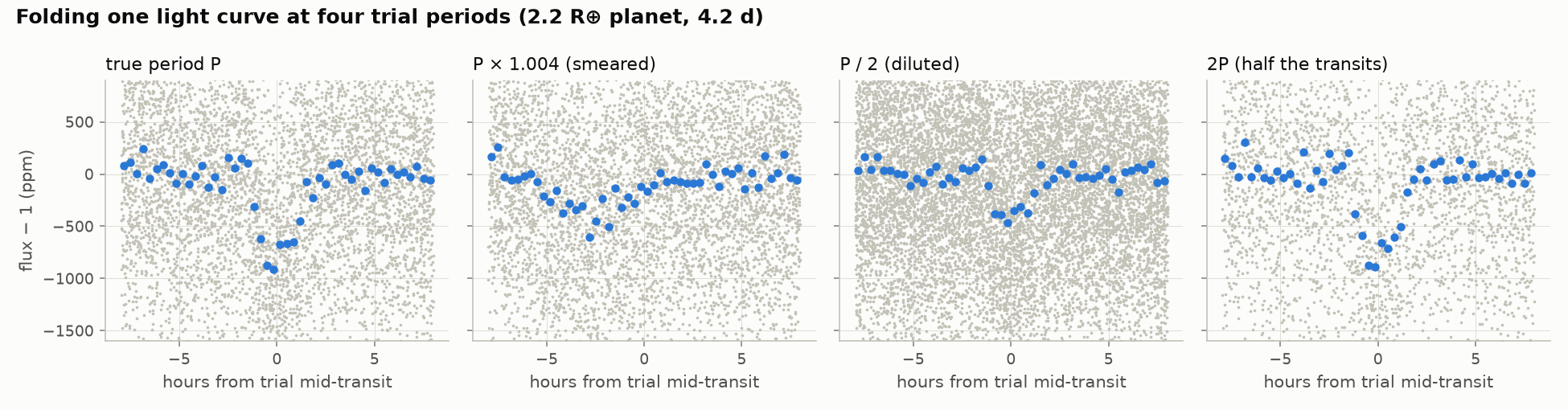
One transit of a small planet is buried in the noise. But transits repeat exactly, so if you guess the right period and phase, you can stack every transit on top of the others. The dip stays the same depth while the noise averages down as \(1/\sqrt{N}\). Guess wrong and the transits smear out or cancel:

Four folded light curves: at the true period a clear dip appears; 0.4 percent off, the dip smears out; at half the period the dip is diluted; at twice the period it is clear but uses half the transits — **Folding one simulated light curve at four trial periods.** At the true period (left) the transits line up. 0.4 % off, they drift apart over the two sectors and smear. At P/2, every other stacked "transit" is empty, which halves the depth. At 2P the dip is clear but only half the transits contribute, so the noise is higher. A search has to tell all of these apart.

Box Least Squares

Box Least Squares (BLS; Kovács, Zucker & Mazeh 2002) makes this systematic. A transit is modeled as a box: flat at level \(y_{\text{out}}\), dropping to \(y_{\text{in}}\) for a duration \(D\) once every period \(P\), starting at phase \(t_0\). For every trial \((P, t_0, D)\) the best-fitting depth and its uncertainty follow from weighted means of the points in and out of the box:

\[\hat\delta = \bar y_{\text{out}} - \bar y_{\text{in}}, \qquad \sigma_\delta^2 = \frac{1}{\sum_{\text{in}} \sigma_i^{-2}} + \frac{1}{\sum_{\text{out}} \sigma_i^{-2}}, \qquad \Delta \ln L = \frac{\hat\delta^{\,2}}{2\,\sigma_\delta^{2}}\]

The improvement in log-likelihood over a flat line. The periodogram plots \(\sqrt{2\,\Delta\ln L} = \hat\delta/\sigma_\delta\), the best over all phases and durations at each period.

Try it. Below is a simulated sector with a hidden 1,300 ppm transit in 900 ppm noise. Drag the trial period and watch the fold, or jump to the highest peak:

Look at the periodogram. The true period makes the tallest peak, but smaller peaks appear at P/2, 2P and other simple fractions of it. These aliases are why the pipeline checks the harmonics of every peak (below).

A grid that knows physics

How many periods need to be tried? If the trial frequency is off by \(\delta f\), transits drift in phase and, over a baseline \(B\), the stack smears by \(B \cdot P \cdot \delta f\) in time. Keeping that smear below a third of the shortest duration \(D_{\min}\) gives a grid that is uniform in log-frequency (Ofir 2014):

\[\delta \ln f = \frac{D_{\min}}{\mathrm{OS} \cdot B}, \qquad \mathrm{OS} = 3\]

Not every duration is possible at every period. For a circular orbit, Kepler’s third law ties the orbit size to the star’s density \(\rho_*\), and that sets the transit duration:

\[\frac{a}{R_*} = \left(\frac{G \rho_* P^2}{3\pi}\right)^{1/3}, \qquad T_{14} \approx \frac{P}{\pi}\,\arcsin\!\left(\frac{R_*}{a}\right)\]

So the period range is split into bands (8 per decade), and each band only tries durations between 0.3× the central duration for the densest plausible star and 1.2× that for the least dense. When the TIC lists the star’s density, densities within a factor of 3 of it are used. Long periods therefore get fewer, longer trial durations, which keeps a three-year search tractable. The search runs on 10-minute bins, then refines the best peak on the unbinned data.

0.6 s1 sector: 12041 trial periods

2.7 s3 sectors: 42991 trial periods

27.7 s13 sectors: 214269 trial periods

142.4 s26 sectors over 3 years: 694018 trial periods

Measured on 4 CPU cores for one search iteration with the stellar density known (full table on the validation page).

Is the peak real? Two statistics

Signal Detection Efficiency. Noise peaks grow with period, because longer periods allow more phases. The pipeline subtracts that slow rise (a running median in log-period bins about 12 % wide), then asks how many standard deviations the peak stands above the rest:

\[\mathrm{SDE} = \frac{\text{peak} - \langle \text{spectrum} \rangle}{\operatorname{std}(\text{spectrum})} \;\ge\; 7\]

Which trials define “the spectrum” matters for long light curves. At every trial period the box can sit on one strong dip, and in a light curve spread thinly over several years, the best box at most long trial periods covers a single dip with the other transits in gaps. Such a trial can never be a detection, which takes two transits, but its scatter would set the scale against which every real signal is measured. So the trend, the mean and the standard deviation come only from trials whose best box holds at least two transits with data. In one to three sectors that is practically every trial (at least 98.8 % in every light curve of the false-alarm calibration), and the calibration’s false-alarm counts came out as before.

Red-noise S/N. White-noise error bars overstate the significance when noise is correlated over hours, as it is for real stars. Instead the pipeline bins the out-of-transit flux into chunks one transit long and measures their scatter \(\sigma_D\) (Pont, Zucker & Queloz 2006), which already contains the correlated part:

\[\mathrm{S/N} = \frac{\hat\delta}{\sigma_D / \sqrt{N_{\text{tr}}}}\]

Paying for the number of trials

A search that tries more combinations gives noise more chances to produce a high peak. The pipeline counts the approximate number of independent trials \(N\) (distinct frequencies × distinct phases × durations counted once per factor of two) and requires a false-alarm probability of \(\alpha = 1\%\) per light curve for Gaussian noise:

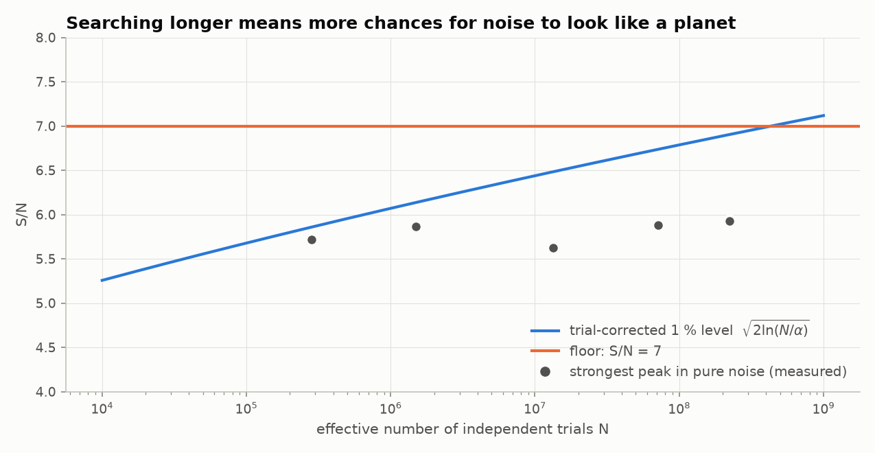
\[\mathrm{S/N}_{\text{threshold}} = \max\!\left(7,\; \sqrt{2 \ln (N/\alpha)}\right)\]

Chart of S/N versus number of trials: the trial-corrected threshold rises slowly from 5.3 to 7.1 as trials grow from ten thousand to a billion; measured noise peaks sit between 5.6 and 6.0, below the floor of 7 — **The threshold rises slowly with the size of the search.** Gray points are the strongest peak found in pure-noise light curves from one sector up to three years (`results/performance/`); all stay below the detection floor of 7, which is comparable to the SPOC pipeline's threshold. Only the longest searches without a density prior push the trial-corrected level above 7.

A peak is a detection if SDE ≥ 7, the red-noise S/N clears the threshold above, and at least two transits fall on data.

Dips at the edges of the data

Real light curves hold dips that no planet made. Most of them sit right after a gap or just before one: after a data downlink the spacecraft settles thermally, scattered light comes and goes, and there the detrending window only sees one side of each point. Such a dip does more harm than one false alarm. Every trial period can put its box on it, so a few strong ones lift the whole periodogram, and two of them, years apart, pair up into a convincing long-period “planet”.

So before each pass the pipeline looks for single dips: for each trial duration, the flux is averaged in boxes centered every quarter-duration, and a box whose average lies at least 7 times its uncertainty below the median is a dip (the uncertainty is the scatter of such averages in the same sector, which includes red noise). A dip is masked like a detected transit if the data do not cover it inside and on both sides, by the same rule as the vetting’s coverage test, and if it lies next to the start or end of a data segment: within 1.5 of its durations, or 6 hours if that is longer, of a gap longer than half a day. A dip left uncovered only because a few cadences are missing in the middle of a segment, near a momentum dump or a run of flagged cadences, is kept.

The first version of the mask did not make that distinction, and it removed real transits. In the validation light curves, 17 of the 22 masked dips that lay far from any long gap were partly covered transits of the planets themselves (WASP-18 b, L 98-59 c and d, pi Men c, TOI-270 c and HD 21749 b). In 2,048 injections into a real light curve, it cost four planets with only two or three transits in the data (Completeness). The current mask recovers three of them. The fourth had a transit 0.8 hours from the end of a segment: a real transit right at the edge of a segment is still masked, but it is one the vetting would not count either.

Choosing among peaks

Peaks are examined from the highest SDE down, skipping trials whose best box holds fewer than two transits with data, and the first one that passes three checks wins:

Harmonic family. P/3, P/2, 2P and 3P are compared, and the search moves to one with a clearly (≥ 1.2×) higher likelihood. For a real transit the likelihood peaks at the true period.
Coverage. At least two transits must contain data.
Starspot test. A spot makes a dip and a bump. A planet only makes a dip. The light curve is folded at the candidate period and averaged in boxes at every phase. If the strongest brightening, at least two durations from the dip, is more than 0.65× as significant as the dip, the peak is skipped as stellar variability. For a transit in white noise the brightest bump is about \(\sqrt{2\ln(P/D)}\,\sigma\), well under half of a 7σ dip. For a pure sinusoid the ratio is 1. (This is a variant of the Kepler Robovetter’s model-shift test, Coughlin et al. 2016.)

Iterating to find every planet

After a detection, its transits are masked, the raw light curve is re-detrended, and the search runs again, up to five times. Each new signal is compared with those already found:

A signal at the same period (or P/2, P/3), whose transits all fall at one phase between the earlier ones, is the other eclipse of the same orbit: a binary’s secondary eclipse or a hot planet’s occultation. The vetting step decides which.
A signal within 0.2 % of an integer ratio of an earlier period and whose transits coincide in time with it is a harmonic and is not counted.
Anything else is a new planet. Both harmonic conditions are needed because real systems sit close to resonance: TOI-270 c and d have periods near 2:1 and must not be merged.

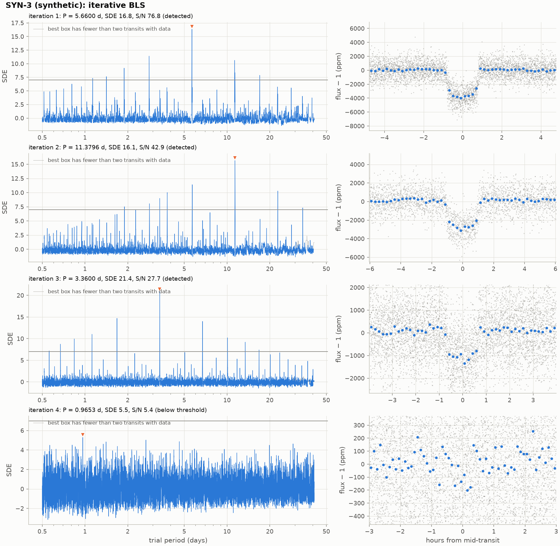
Four rows of BLS periodograms with folded transits: three iterations find planets at 5.66, 11.38 and 3.36 days; the fourth finds nothing above threshold — **Iterative search on SYN-3, a simulated three-planet M-dwarf system.** Each row is one pass: periodogram with the SDE = 7 line (left) and the fold at the chosen peak (right). The planets are found in order of signal strength: 5.66 d (S/N 76.8), 11.38 d (S/N 42.9) and 3.36 d (S/N 27.7). The fourth pass peaks at SDE 5.5, below threshold, so the search stops.

SYN-3 was built with the periods of a real system, TOI-270. The same search on seven sectors of its TESS data:

Five rows of BLS periodograms for TOI-270: three strong detections at 5.66, 11.38 and 3.36 days, then two weak ones at 46.67 and 88.84 days whose folds are noisy — **Iterative search on TOI-270 (TESS data).** The three known planets come out in the same order as in the simulation: 5.66 d (S/N 89.4), 11.38 d (S/N 55.3) and 3.36 d (S/N 31.3). The fourth and fifth passes just clear both thresholds, at 46.67 d (SDE 7.5, S/N 9.3) and 88.84 d (SDE 7.6, S/N 8.2), and the vetting rejects both: all three "transits" of the first sit at the edges of gaps in the data (coverage test), and the second's odd and even transits differ by 4.4σ. The search stops there, at its limit of five passes. 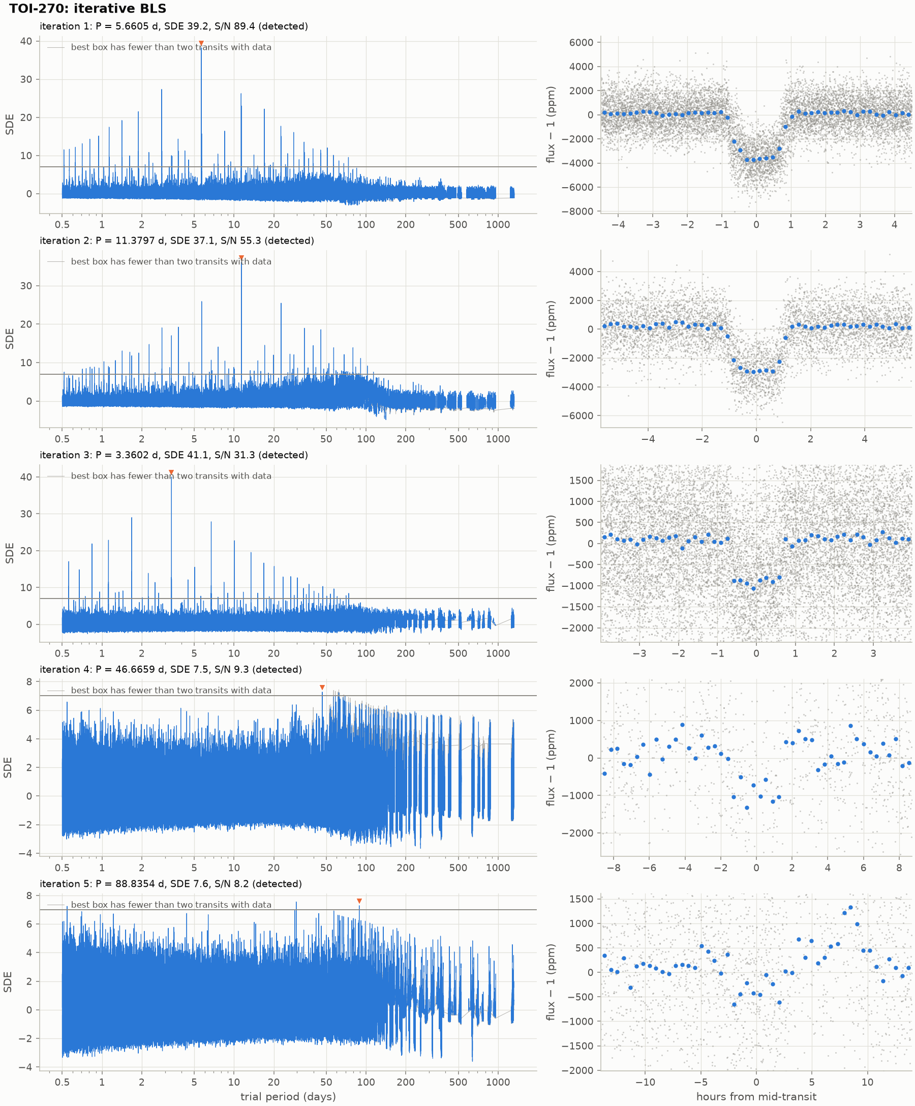Values from `results/validation/TOI-270/summary.md`.