Measuring what you miss
Finding nothing around a star doesn’t mean there’s nothing there. To say what the search could have found, you plant fake planets in the data and see how many come back. The fraction recovered is the pipeline’s completeness, and every planet-occurrence rate or “no planet larger than X” claim depends on it.
The procedure
- Draw a planet in a period × radius cell: period and radius log-uniform within the cell, impact parameter uniform in [0, 0.9], epoch uniform within the first period, circular orbit around the host’s mass and radius.
- Multiply its batman model into the light curve before detrending, so any damage the detrending does to transits counts against the pipeline.
- Run the same detrend and iterative search (two iterations) as for a real star.
- Count it as recovered if a detected signal matches in both period and time:
Detections at 1/3, 1/2, 2 or 3 times the period that line up in time are recorded as aliases and not counted.
Each cell’s completeness is a binomial fraction, with uncertainty
\[C = \frac{n_{\text{rec}}}{n_{\text{inj}}}, \qquad \sigma_C \approx \sqrt{\frac{C(1-C)}{n_{\text{inj}}}},\]so with 32 injections per cell a 50 % cell is known to about ±9 %.
The completeness map
For a simulated two-sector light curve of a Sun-like star with 140 ppm of scatter per hour. Hover over a cell for the counts.
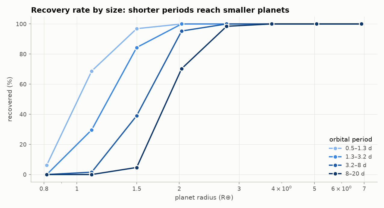
Why the boundary is where it is
The shape of the map follows from the signal-to-noise of a stacked transit. With \(N_{\text{tr}} \approx B/P\) transits of duration \(T_{14} \propto P^{1/3}\):
So at fixed S/N the smallest detectable planet grows only slowly with period, as \(R_p \propto P^{1/6}\). Doubling the data lowers it by a factor \(2^{1/4} \approx 1.19\).
You can explore the same formula with the calculator on the home page.
An upper limit
The simulated light curve has starspots and correlated noise but no spacecraft systematics
(momentum dumps, scattered light), so this map is an upper limit on real-data
completeness at the same noise level. The same script runs on real stars with their known
planets masked (--tic <ID> --mask-known). The completeness page
has the map for two sectors of HD 21749, and what it does and does not show.