From a box to a planet
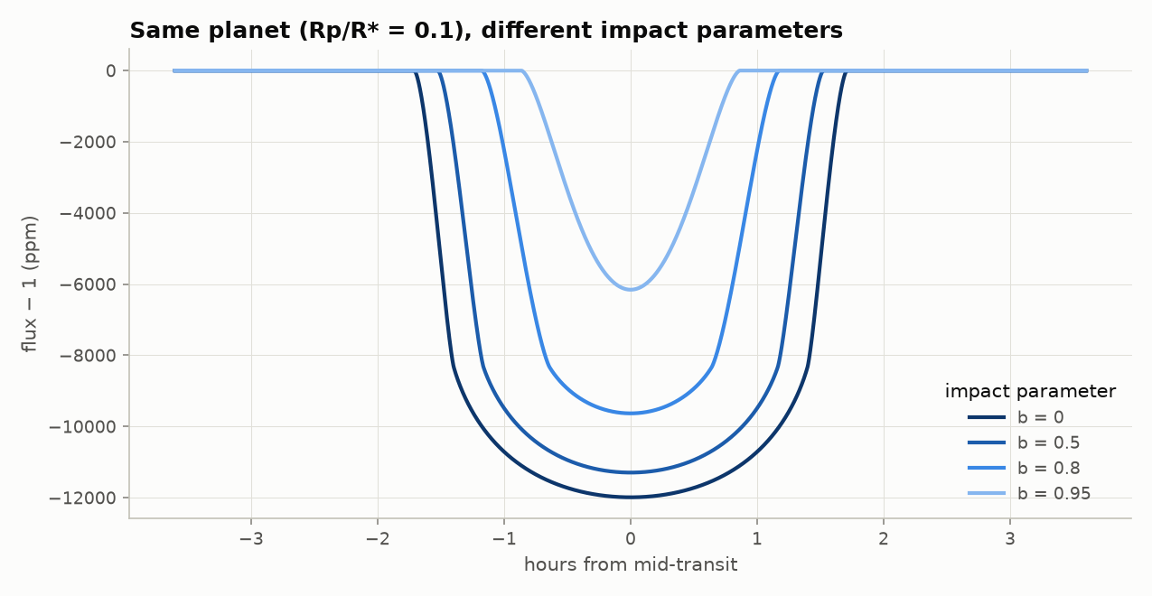
BLS finds a box. A real transit isn’t box-shaped: the planet takes time to cross the star’s edge (ingress and egress), and the star is dimmer at its limb than at its center, which rounds the bottom. Fitting a physical model to that shape gives the planet’s size, the geometry of its orbit and, through Kepler’s laws, the density of its star.
The model is batman (Kreidberg 2015): the exact flux blocked by an opaque disk crossing a limb-darkened star on a circular orbit. The star’s brightness profile is quadratic in \(\mu = \cos\theta\), the angle between the line of sight and the surface normal:
\[\frac{I(\mu)}{I(1)} = 1 - u_1(1-\mu) - u_2(1-\mu)^2\]What the shape tells you
| parameter | what it controls | prior |
|---|---|---|
| \(T_0\) | time of mid-transit | uniform, ±1 BLS duration |
| \(P\) | period | uniform, ±(duration × P / time span) |
| \(k = R_p/R_*\) | depth ≈ \(k^2\) | uniform (10⁻⁴, 1) |
| \(\ln(a/R_*)\) | duration, via orbital speed | uniform (ln 1.2, ln 500) |
| \(b\) | ingress/egress length, chord | uniform (0, 1 + k) |
| \(q_1, q_2\) | limb darkening | uniform (0, 1) |
| \(f_0\) | out-of-transit baseline | uniform (0.9, 1.1) |
| \(\ln \sigma_{\text{jit}}\) | extra white noise | uniform (ln 10⁻⁷, ln 0.1) |
The limb-darkening coefficients are sampled in the Kipping (2013) parameterization,
\[u_1 = 2\sqrt{q_1}\,q_2, \qquad u_2 = \sqrt{q_1}\,(1 - 2q_2),\]which maps the unit square exactly onto the physically allowed laws (brightness positive everywhere and decreasing toward the limb), so uniform priors on \(q_1, q_2\) are uninformative.
The likelihood
Only data within ±2.5 durations of each transit are fitted, with the other planets’ transits removed. Each point’s error bar is inflated by a jitter term that the fit learns:
Sampling with MCMC
The posterior is explored with emcee (Foreman-Mackey et al. 2013), an affine-invariant ensemble sampler. 40 walkers start near the maximum-a-posteriori point, found by optimizing from three impact parameters (0.1, 0.5, 0.8) so as not to get stuck in a grazing or non-grazing local optimum.
A chain is treated as converged when it is longer than 50 integrated autocorrelation times \(\tau\) and the estimate of \(\tau\) has changed by less than 1 % (checked every 500 steps, 2,000 to 20,000 steps). Burn-in is \(2\tau\) and the chain is thinned by \(\tau/2\). Shallow transits often hit the step limit first, because \(b\), \(a/R_*\), \(k\) and limb darkening are strongly correlated. Every report says so when that happens.
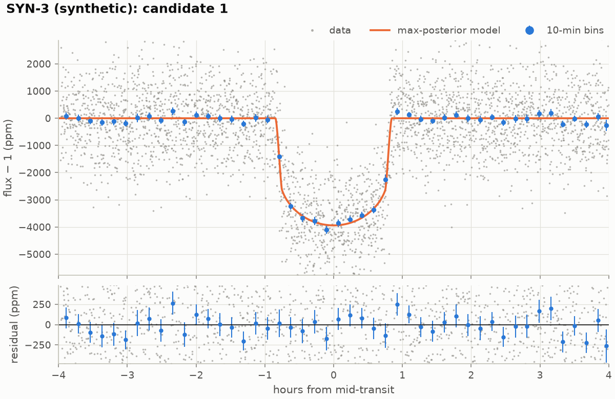
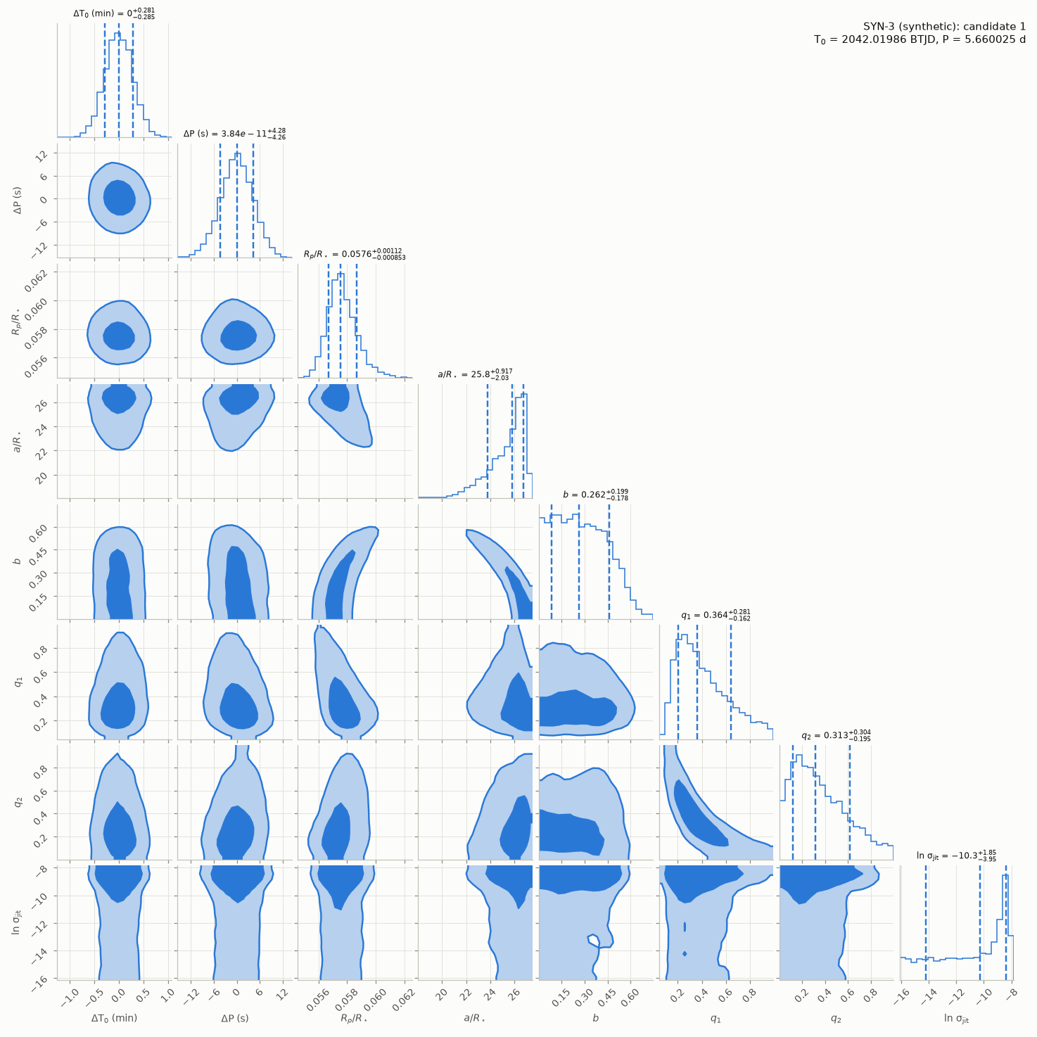
SYN-3 c, fitted. Left: the folded data, 10-minute bins and the best model, with residuals. Right: the posterior. The banana-shaped correlations between b, a/R* and k are why shallow transits need long chains.
Derived properties
Everything below is computed sample by sample from the chain, so uncertainties propagate automatically. Reported values are posterior medians with 68 % intervals.
The planet radius uses the TIC stellar radius, with its catalog uncertainty drawn into every sample. \(T_{\text{eq}}\) assumes zero albedo and full heat redistribution.
Why the star’s density is not a prior Most transit fitters tie \(a/R_*\) to the catalog stellar density. This one deliberately doesn’t. The density implied by the transit shape is then an independent measurement, and comparing it with the catalog is one of the strongest tests for impostors (Vet).